1
2
3
4
5
6
7
8
9
10
11
12
13
14
15
16
17
18
19
20
21
22
23
24
25
26
27
28
29
30
31
32
33
34
35
36
37
38
39
40
41
42
43
44
45
46
47
48
49
50
51
52
53
54
55
56
57
58
59
60
61
62
63
64
65
66
67
68
69
70
71
72
73
74
75
76
77
78
79
80
81
82
83
84
85
86
87
88
89
90
91
92
93
94
95
96
97
98
99
100
101
102
103
104
105
106
107
108
109
110
111
112
113
114
115
116
117
118
119
120
121
122
123
124
125
|
cd "D:\Data Storages\Dataset for Learning"
use nlsy.dta,clear
gen id= _n
reshape long anti self pov, i(id)
bys id:gen times = _n
set matsize 11000

xtset id
xtreg anti,mle

------------------------------------------------------------------------------
        anti |      Coef.   Std. Err.      z    P>|z|     [95% Conf. Interval]
-------------+----------------------------------------------------------------
       _cons |   1.636833   .0557054    29.38   0.000     1.527652    1.746014
-------------+----------------------------------------------------------------
    /sigma_u |   1.208859   .0441422                      1.125365    1.298547
    /sigma_e |    1.01226   .0209977                      .9719306    1.054263
         rho |   .5878254   .0214793                      .5453008    .6293423
------------------------------------------------------------------------------
LR test of sigma_u=0: chibar2(01) = 578.26             Prob >= chibar2 = 0.000

dis e(sigma_u)^2
1.4613398

dis e(sigma_e)^2
1.0246701

mixed anti || id:, mle
eststo m1

------------------------------------------------------------------------------
        anti |      Coef.   Std. Err.      z    P>|z|     [95% Conf. Interval]
-------------+----------------------------------------------------------------
       _cons |   1.636833   .0557054    29.38   0.000     1.527652    1.746014
------------------------------------------------------------------------------


------------------------------------------------------------------------------
  Random-effects Parameters  |   Estimate   Std. Err.     [95% Conf. Interval]
-----------------------------+------------------------------------------------
id: Identity                 |
                  var(_cons) |   1.461341   .1067235      1.266447    1.686226
-----------------------------+------------------------------------------------
               var(Residual) |    1.02467   .0425105      .9446484     1.11147
------------------------------------------------------------------------------
LR test vs. linear model: chibar2(01) = 578.26        Prob >= chibar2 = 0.0000

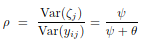
ICC(intraclass correlation coefficient)= var(_cons)/[var(_cons)+var(Residual)] = 1.461341 / (1.461341+1.02467) = .58782564
组内相关系数为58.78%,表明有58.78%的变异是由研究对象差异(组间斜率差异)造成

estat icc

Intraclass correlation

------------------------------------------------------------------------------
                       Level |        ICC   Std. Err.     [95% Conf. Interval]
-----------------------------+------------------------------------------------
                          id |   .5878256   .0214794      .5451833    .6291892
------------------------------------------------------------------------------


mean anti

Mean estimation                   Number of obs   =      1,743

--------------------------------------------------------------
             |       Mean   Std. Err.     [95% Conf. Interval]
-------------+------------------------------------------------
        anti |   1.636833    .037777       1.56274    1.710926
--------------------------------------------------------------

reg anti
eststo m2

      Source |       SS           df       MS      Number of obs   =     1,743
-------------+----------------------------------   F(0, 1742)      =      0.00
       Model |           0         0           .   Prob > F        =         .
    Residual |  4333.11532     1,742  2.48743704   R-squared       =    0.0000
-------------+----------------------------------   Adj R-squared   =    0.0000
       Total |  4333.11532     1,742  2.48743704   Root MSE        =    1.5772


------------------------------------------------------------------------------
        anti |      Coef.   Std. Err.      t    P>|t|     [95% Conf. Interval]
-------------+----------------------------------------------------------------
       _cons |   1.636833    .037777    43.33   0.000      1.56274    1.710926
------------------------------------------------------------------------------

mixed anti
eststo m3

Mixed-effects ML regression                     Number of obs     =      1,743


                                                Wald chi2(0)      =          .
Log likelihood = -3266.8666                     Prob > chi2       =          .


------------------------------------------------------------------------------
        anti |      Coef.   Std. Err.      z    P>|z|     [95% Conf. Interval]
-------------+----------------------------------------------------------------
       _cons |   1.636833   .0377662    43.34   0.000     1.562813    1.710853
------------------------------------------------------------------------------


------------------------------------------------------------------------------
  Random-effects Parameters  |   Estimate   Std. Err.     [95% Conf. Interval]
-----------------------------+------------------------------------------------
               var(Residual) |    2.48601   .0842111      2.326319    2.656663
------------------------------------------------------------------------------

lrtest m1 m3, stats

Likelihood-ratio test                                 LR chi2(1)  =    578.26
(Assumption: m3 nested in m1)                         Prob > chi2 =    0.0000

-----------------------------------------------------------------------------
       Model |          N   ll(null)  ll(model)      df        AIC        BIC
-------------+---------------------------------------------------------------
          m3 |      1,743          .  -3266.867       2   6537.733    6548.66
          m1 |      1,743          .  -2977.735       3    5961.47   5977.861
-----------------------------------------------------------------------------
Note: BIC uses N = number of observations. See [R] BIC note.
|