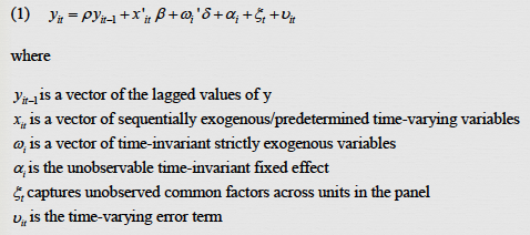
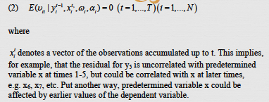
利用最大似然法估计固定效应交叉滞后面板模型

  • Allison, P. D., Williams, R., & Moral-Benito, E. (2017). Maximum likelihood for cross-lagged panel models with fixed effects. Socius, 3, 2378023117710578.
  • 常见Stata包
    • xtabond:Arellano-Bond linear dynamic panel-data estimation
    • xtabond2:"Difference" and "system" generalized method-of-moments (GMM) dynamic panel estimator
    • xtdpd:Linear dynamic panel-data estimation
    • xtdpdsys:Arellano-Bover/Blundell-Bond linear dynamic panel-data estimation
    • xtdpd: Linear dynamic panel-data estimation
    • xtdpdqml:Quasi-maximum likelihood linear dynamic panel-data estimation
    • xtdpdml:Dynamic panel-data models using maximum likelihood
    • xtdpdbc:Bias-corrected estimation of linear dynamic panel models
    • xtdpdgmm:GMM estimation of linear dynamic panel models
    • xtlsdvc:Bias corrected LSDV dynamic panel data estimator
    • fect:A Practical Guide to Counterfactual Estimators for Causal Inference with Time-Series Cross-Sectional Data
    • 结合使用最大似然法与结构方程模型,简称ML-SEM
    • 在大部分条件下,ML-SEM比GMM更有效,且偏误更小
  • R 包
  • 面板数据(追踪数据或TSCS数据)对非实验数据做出因果推断具有两大优势
    • 能够控制不被观测到的,非时混淆因素
      • 使用固定效应模型
    • 考虑滞后期互为因果关系,确定因果关系的方向
      • 第t期x和y能够同时影响第t+1期的x和y
      • 使用交叉滞后面板模型(cross-lagged panel model),源于Duncan的二期双变量模型(two-wave,two variable model)
  • 同时解决未观测混淆因素与确定因果关系方向的问题
    • 结合固定效应模型和交叉滞后面板模型存在严重的估计问题
      • 由于因变量的滞后效应,计量经济学把这类模型称为动态面板模型(dynamic panel data)
    • 动态面板模型的估计难题
      • 误差项与预测变量相关
      • 偶然参数问题(incidental parameters problem)
      • 干预变量初始条件的非确定性(uncertainties about the treatment of initial conditions)
    • 估计动态面板模型的方法
      • 把滞后期变量作为工具变量,即滞后期工具变量(lagged instrumental variable),进行广义矩估计方法(generalized method of moment,简称GMM)
      • 通常使用Arellano-Bond估计法(AB estimator)
        • xtabond、xtabond2
    • 虽然AB方法为系数提供了一致估计,并非完全有效
      • 存在相当大的小样本偏差
      • 自回归参数(autoregressive)接近1时表现不佳
        • 即因变量在以后某个时点对自身的影响
    • Moral-Benito和白聚山的看法
      • 采用最大似然法(Maximum Likelihood Estimation)可以克服偶然参数问题和初始条件问题
      • 以Moral-Benito(2013)为顶峰,有效解决动态面板模型的估计问题
  • Moral-Benito方法
    • 条件2需要一致性和渐进正态性
    • Moral-Benito方法并未包括严格外生的时变变量,但可以修改加入
  • Allison(2014)证明了动态面板模型是广义线性结构方程模型(general linear structural equation model)的特殊案例
  • Allison和Moral-Benito(2013)证明SEM方法相比于GMM方法和早前ML方法的优点
    • 不存在偶然参数问题
    • 初始条件作为完全外生的变量,不必纳入模型
    • 当自回归参数接近1时,不存在估计问题
    • 基于完全信息的最大似然估计(full information maximum likelihood,FIML)可以解决预测变量的缺失值问题
    • 允许误差项方差随时间变化
    • 允许不可观测的、非时变因素的效应
      • AB方法不行,将差分掉
    • 许多模型限制可以很容易放松或检验
    • 可以使用许多拟合优度测量法来评估模型的过度识别问题
    • 不必在许多工具变量中进行选择
    • 可以将多个指标的潜变量纳入模型
    • 可以将非时变变量纳入模型
  • xtdpdml计算的优势
    • 简化SEM建模
    • 所有的变量效应被认为在不同时期相等
    • LR统计量提供总体拟合优度检验
    • wald统计量检验模型中的任何变量效应是否显著区别于0
  • Moral-Benito(2013)方法的局限
    • 可能存在收敛失败
    • 计算慢于AB方法,特别是使用FIML处理非平衡形式的缺失数据时
  • 交叉滞后面板模型与动态面板模型的比较
    • 交叉滞后面板模型
      • w和z被认为是严格外生的
    • 动态面板模型
      • 基本与交叉滞后面板模型相似
      • x通常是一个向量而非标量
      • x通常不会滞后
      • αj被视为一组固定常数而非一组随机变量
        • 等价于允许α与所有时变预测变量之间存在无限制的相关性
    • 交叉滞后面板模型是动态面板模型的特例
      • 动态面板模型->交叉滞后面板模型
      • 滞后x并将其从一个向量减少到一个标量
      • 将固定效应转变为随机效应
      • 将方程2的结构强加于x对滞后y的依赖关系中
  • Arellano-Bond的广义矩估计法存在的问题
    • 小样本偏误
    • 低效率
    • 选择工具变量的不确定性
  • ML-SEM方法与AB方法的比较
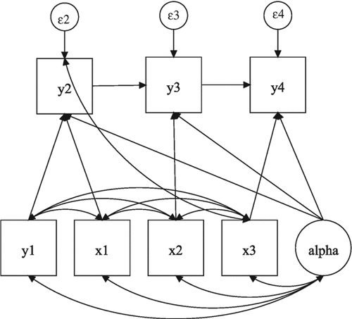
    • 四期动态面板模型的路径图
    • ML-SEM提出更强有力的预设
      • 所有内生变量都是正态多元
      • cov(ε, z) = 0
    • ML-SEM也放松很多AB方法的预设
      • 允许时间变量本身不受限制的影响
      • 允许每个时间点上有不同的误差方差
      • 允许个体效应的潜在变量α在不同时间点有不同的系数
      • 允许固定效应与时变预测变量有不受限制的相关性,不依赖差分和其他方法消除固定效应
      • 允许误差项与时变预测变量的未来取值相关
      • 许多参数在不同时期的固定条件,可以被放松
    • MB方法总体在一致估计和有效估计方面优于AB方法,且还有几个其他优点
      • 非时变变量可以纳入模型中
      • 完全信息最大似然法(FIML)可以很容易处理预测变量中的缺失值
      • 误差方差和其他参数可以随时间变化
      • 可以使用许多拟合优度测量方法来评估模型的过度识辨限制
      • 没有必要在许多可能的工具变量中进行选择
  • 案例Cornwell and Rupert (1988)
 1
 2
 3
 4
 5
 6
 7
 8
 9
10
11
12
13
14
15
16
17
18
19
20
21
22
23
24
25

use https://www3.nd.edu/~rwilliam/statafiles/wages, clear
xtset id t
eststo m1: xtdpdml wks L.lwage, pre(L.union) inv(ed) errorinv lavaan(Socius, r)
esttab m1, nogap se
----------------------------
                      (1)   
                      wks   
----------------------------
wks2                        
wks1                0.188***
                 (0.0196)   
lwage1              0.588   
                  (0.488)   
union1             -1.206*  
                  (0.522)   
ed                 -0.107   
                 (0.0564)   
Alpha               1.000***
               (5.07e-16)   
E2                  1.000***
               (6.69e-16)   
_cons               36.37***
                  (2.893)   
----------------------------
  • 案例Bollen & Brand(2010)
    • Bollen, K. A., & Brand, J. E. (2010). A general panel model with random and fixed effects: A structural equations approach. Social Forces, 89(1), 1-34.
 1
 2
 3
 4
 5
 6
 7
 8
 9
10
11
12
13
14
15
16
17
18
19
20
21
22
23
24
25
26
27
28
29
30
31
32
33
34
35
36

cd "/Users/ginglam/OneDrive - whu.edu.cn/07_Scholars/Jennie E. Brand/A General Panel Model with Random and Fixed Effects/"
use bollenbrand.dta,clear
xtset id year

qui: eststo m1: xtreg lnwg hchild i.year
qui: eststo m2: xtreg lnwg hchild marr div i.year
qui: eststo m3: xtreg lnwg hchild marr div eduatt cursc snrpt snrft exppt expft break i.year
qui: eststo m4: xtreg lnwg hchild i.year, fe
qui: eststo m5: xtreg lnwg hchild marr div i.year, fe
qui: eststo m6: xtreg lnwg hchild marr div eduatt cursc snrpt snrft exppt expft break i.year, fe
esttab m1 m2 m3 m4 m5 m6, nogap se keep(hchild)

------------------------------------------------------------------------------------------------------------
                      (1)             (2)             (3)             (4)             (5)             (6)   
                     lnwg            lnwg            lnwg            lnwg            lnwg            lnwg   
------------------------------------------------------------------------------------------------------------
hchild            -0.0876***      -0.0963***      -0.0343***      -0.0646***      -0.0691***      -0.0436***
                (0.00399)       (0.00409)       (0.00391)       (0.00560)       (0.00564)       (0.00563)   
------------------------------------------------------------------------------------------------------------
N                   20841           20841           20841           20841           20841           20841   
------------------------------------------------------------------------------------------------------------
Standard errors in parentheses
* p<0.05, ** p<0.01, *** p<0.001


use bollenbrand.dta,clear
qui: eststo m7: xtdpdml lnwg hchild, ylag(0) re fiml tfix errorinv 
qui: eststo m8: xtdpdml lnwg hchild marr div, ylag(0) re fiml tfix errorinv
qui: eststo m9: xtdpdml lnwg hchild marr div eduatt cursc snrpt snrft exppt expft break , ylag(0) re fiml tfix errorinv
qui: eststo m10: xtdpdml lnwg hchild, ylag(0) fiml tfix errorinv
qui: eststo m11: xtdpdml lnwg hchild marr div, ylag(0) fiml tfix errorinv
qui: eststo m12: xtdpdml lnwg hchild marr div eduatt cursc snrpt snrft exppt expft break , ylag(0) fiml tfix errorinv
esttab m7 m8 m9 m10 m11 m12, nogap se keep(hchild1)

------------------------------------------------------------------------------------------------------------                      (1)             (2)             (3)             (4)             (5)             (6)                        lnwg            lnwg            lnwg            lnwg            lnwg            lnwg   ------------------------------------------------------------------------------------------------------------lnwg1                                                                                                       hchild1           -0.0877***      -0.0965***      -0.0342***      -0.0659***      -0.0705***      -0.0433***                (0.00399)       (0.00409)       (0.00390)       (0.00557)       (0.00559)       (0.00557)   ------------------------------------------------------------------------------------------------------------N                    5231            5231            5231            5231            5231            5231   ------------------------------------------------------------------------------------------------------------Standard errors in parentheses* p<0.05, ** p<0.01, *** p<0.001
  • xtdpdml与xtabond的比较
    • xtabond预设恒定截距(constant intercept)和恒定方差(constant variance)
      • xtdpdml可以设定constinv与errorinv来确保与xtabond的可比性,但这些预设是没有必要的
      • xtabond删除了所有包含确实数据的样本,因而在缺失数据中得到难以置信的估计结果
    • 在数据远没有强烈平衡的情况下,xtabond运行得更好或xtdpdml可能无法执行
    • 如果模型有许多缺失数据和非时变变量,xtdpdml是更好的选择
      • xtdpdml显示的是每一期的样本量,而非全部样本量
      • xtdpdml可以缺省fiml,删除缺失值样本以得到与xtabond相似的估计环境
 1
 2
 3
 4
 5
 6
 7
 8
 9
10
11
12
13
14
15
16
17
18

eststo m14: xtabond lnwg hchild marr div eduatt cursc snrpt snrft exppt expft break black hisp
eststo m15: xtdpdml lnwg hchild marr div eduatt cursc snrpt snrft exppt expft break, constinv errorinv fiml tfix store(fiml) inv(black hisp)
eststo m16: xtdpdml lnwg hchild marr div eduatt cursc snrpt snrft exppt expft break, constinv errorinv tfix store(fiml) inv(black hisp)
 esttab m14 m15 m16,nogap se keep(hchild hchild2)

------------------------------------------------------------
                      (1)             (2)             (3)   
                     lnwg            lnwg            lnwg   
------------------------------------------------------------
main                                                        
hchild           -0.00913                                   
                (0.00906)                                   
hchild2                           -0.0210***      -0.0145   
                                (0.00636)       (0.00998)   
------------------------------------------------------------
N                    8915            5285            1229   
------------------------------------------------------------
  • 拟合优度的衡量(goodness-of-fit measures)
    • 检查α系数(未测量的固定效应系数)在不同时间段是否相同
      • 检验4、8、12、16、20、21表明,α在不同时间段并不相同
    • 检验误差方差(error variances)在不同时间段是否相同(errorinv选项设定为相同,但该约束是可疑的)
      • 检验22、23、24表明,误差方差在不同时间段不同
    • 与AB估计法不同,以上两个问题都可以用ML-SEM估计法解决
      • AIC和BIC结果也支持约束更少的模型
 1
 2
 3
 4
 5
 6
 7
 8
 9
10
11
12
13
14
15
16
17
18
19
20
21
22
23
24
25
26
27
28
29
30
31
32
33
34
35
36
37
38
39
40
41
42
43
44
45
46
47
48
49
50
51
52
53
54
55
56
57
58
59
60
61
62
63

eststo m17: xtdpdml lnwg hchild marr div, ylags(0) fiml tfix errorinv gof store(m17)
esttab m17, nogap se scalar(chi2_ms df_ms p_ms BIC AIC) keep(hchild1)

----------------------------
                      (1)   
                     lnwg   
----------------------------
lnwg1                       
hchild1           -0.0705***
                (0.00559)   
----------------------------
N                    5231   
chi2_ms            1940.9   
df_ms                 106   
p_ms                    0   
BIC               73683.2   
AIC               72252.6   
----------------------------

estat scoretests

  ( 1)  [lnwg1]hchild1 - [lnwg6]hchild6 = 0  ( 2)  [lnwg1]marr1 - [lnwg6]marr6 = 0  ( 3)  [lnwg1]div1 - [lnwg6]div6 = 0  ( 4)  [lnwg1]Alpha = 1  ( 5)  [lnwg2]hchild2 - [lnwg6]hchild6 = 0  ( 6)  [lnwg2]marr2 - [lnwg6]marr6 = 0  ( 7)  [lnwg2]div2 - [lnwg6]div6 = 0  ( 8)  [lnwg2]Alpha = 1  (12)  [lnwg3]Alpha = 1  (13)  [lnwg4]hchild4 - [lnwg6]hchild6 = 0  (15)  [lnwg4]div4 - [lnwg6]div6 = 0  (16)  [lnwg4]Alpha = 1  (17)  [lnwg5]hchild5 - [lnwg6]hchild6 = 0  (20)  [lnwg5]Alpha = 1  (21)  [lnwg6]Alpha = 1  (22)  [var(e.lnwg1)]_cons - [var(e.lnwg6)]_cons = 0  (23)  [var(e.lnwg2)]_cons - [var(e.lnwg6)]_cons = 0  (24)  [var(e.lnwg3)]_cons - [var(e.lnwg6)]_cons = 0---------------------------------------             |      chi2     df  P>chi2-------------+-------------------------        ( 1) |    54.652      1    0.00        ( 2) |    17.970      1    0.00        ( 3) |     4.194      1    0.04        ( 4) |   543.286      1    0.00        ( 5) |    15.011      1    0.00        ( 6) |     5.726      1    0.02        ( 7) |     8.885      1    0.00        ( 8) |    91.101      1    0.00        (12) |     5.594      1    0.02        (13) |     5.866      1    0.02        (15) |     4.213      1    0.04        (16) |    98.223      1    0.00        (17) |     4.062      1    0.04        (20) |   100.611      1    0.00        (21) |   134.406      1    0.00        (22) |    12.887      1    0.00        (23) |    20.007      1    0.00        (24) |    20.581      1    0.00———————————————————

*修正后的模型,许可α和误差方差随时间变化
eststo m18: xtdpdml lnwg hchild marr div, ylags(0) fiml tfix alphafree gof store(m18)
esttab m18, nogap se scalar(chi2_ms df_ms p_ms BIC AIC) keep(hchild1)

----------------------------
                      (1)   
                     lnwg   
----------------------------
lnwg1                       
hchild1           -0.0455***
                (0.00579)   
----------------------------
N                    5231   
chi2_ms             789.3   
df_ms                  96   
p_ms            1.90e-109   
BIC               72617.2   
AIC               71120.9   
----------------------------
Standard errors in parentheses

lrtest m17 m18, stats

Likelihood-ratio test
Assumption: m17 nested within m18

LR chi2(10) = 1151.68
Prob > chi2 =  0.0000

Akaike's information criterion and Bayesian information criterion

-----------------------------------------------------------------------------
       Model |          N   ll(null)  ll(model)      df        AIC        BIC
-------------+---------------------------------------------------------------
         m17 |      5,231          .  -35908.31     218   72252.61   73683.21
         m18 |      5,231          .  -35332.47     228   71120.93   72617.15
-----------------------------------------------------------------------------
Note: BIC uses N = number of observations. See [R] BIC note.

  • 固定效应与随机效应的似然比检验(likelihood-ratio test)
    • 使用lrtest re fe, stats
    • Allison (2009)指出,豪斯曼检验经常出现问题,比如产生负值
    • 似然比检验具有优越的统计特性
 1
 2
 3
 4
 5
 6
 7
 8
 9
10
11
12
13
14
15
16
17
18

lrtest m9 m12, stats

Likelihood-ratio test
Assumption: m9 nested within m12

LR chi2(60) = 337.14
Prob > chi2 = 0.0000

Akaike's information criterion and Bayesian information criterion

-----------------------------------------------------------------------------
       Model |          N   ll(null)  ll(model)      df        AIC        BIC
-------------+---------------------------------------------------------------
          m9 |      5,231          .  -184555.8    1908   372927.6   385448.6
         m12 |      5,231          .  -184387.2    1968   372710.4   385625.2
-----------------------------------------------------------------------------
Note: BIC uses N = number of observations. See [R] BIC note.
  • 使用稳健标准误
    • vce (sbentler)不能与fiml一起使用
    • vce(robust)可以同fiml一起使用
1
2
3

xtdpdml lnwg hchild marr div eduatt cursc snrpt snrft exppt expft break, constinv errorinv tfix vce(sbentler) inv(black hisp) gof
xtdpdml lnwg hchild marr div eduatt cursc snrpt snrft exppt expft break, constinv errorinv tfix inv(black hisp) vce(robust) gof