增长曲线模型-教材 | Stata

  • Multilevel and Longitudinal Modeling using Stata
  • 增长曲线模型(growth-curve models)
    • 多层次分析方法的一种
    • 又称为潜在轨迹模型(latent-trajectory models)或潜在增长曲线模型(latent growth-curve models)
    • 可以对个体特征随事件的轨迹及轨迹的变化进行建模。
    • 本质上是对个体内变化的个体间差异建模
  • 增长曲线模型与随机系数模型(random-coefficient model)的关系
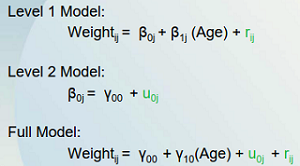
    • 增长曲线模型是随机系数模型的特殊案例,表现在时间系数(一般是年龄)随个体而变化

    • 潜在增长模型是描述和解释个体随时间变化的技术
    • 关注问题
      • 个体随时间(年龄)变化的模式是怎样的?
      • 如何解释个体随时间(年龄)变化的模式?
    • 数据要求
      • 面板数据,至少3期
      • 结果变量被重复测量3次
      • 必须有时间变量
      • 面板期数越长,可以估计的模型复杂度越高。
        • 三期数据可以估计线性增长曲线模型。
        • 四期数据可以估计线性和非线性增长曲线模型。
        • 函数形式由研究者根据数据实际情况定义
    • 主要任务
      • 对个体内变化建模(model intra-individual change):同一个人的结果变量在不同时期的变化,时间是唯一的预测变量,结果变量的变化与时间之间的关系称为轨迹(trajectory);
        • 解释轨迹是否是线性、曲线、立方和其他函数形式
        • 定义轨迹的时间参数是否具有显著异变异
      • 解释个体轨迹在不同个体间的差异(explain inter-individual differences in the intra-individual trajectories):个体间的差异可以作为预测变量,解释个体变化轨迹的异质性
        • 使用非时变和时变变量来解释轨迹参数的变异
    • 关键概念:轨迹(trajectory)
      • 轨迹是个体随时间变化的模式(patterns of change for individuals over time)
      • 轨迹是关于时间的函数(function of time)
        • 不同的轨迹代表时间与关键变量存在不同函数形式
      • 轨迹可以呈现为不同函数形式,包括线性、曲线、立方和其他形式
      • 轨迹描述个体是否随时间变化且变化有多快
      • 高阶函数形式需要更多参数
        • 研究人们为何有不同的轨迹,等同于检验不同属性的人们是否有不同轨迹,即个体内变化模式的个体间差异
        • 如果人们的轨迹不同,意味着他们至少在定义轨迹的一个参数上存在差异
    • gllamm用法
1
2
3
4
5
6

use "/Users/ginglam/Onedrive/02_Data_Storages/Dataset for Learning/childweight.dta",clear
global MLwiN_path "C:\Program Files\MLwiN v3.00\mlwin.exe"
set scheme s1mono
bys id (age):gen newid = _n
gen cons = 1
  • 传统回归模型
 1
 2
 3
 4
 5
 6
 7
 8
 9
10
11
12
13
14
15
16
17
18
19
20
21
22
23
24
25
26
27
28
29
30
31
32
33

reg weight age
eststo m1
mixed weight age,  nolog
eststo m2
esttab m1 m2,nogap

--------------------------------------------
                      (1)             (2)   
                   weight          weight   
--------------------------------------------
main                                        
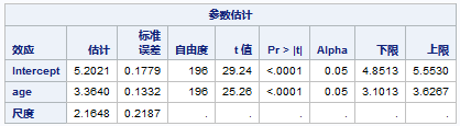
age                 3.364***        3.364***
                  (25.26)         (25.39)   
_cons               5.202***        5.202***
                  (29.24)         (29.39)   
--------------------------------------------
lnsig_e                                     
_cons                               0.381***
                                   (7.58)   
--------------------------------------------
N                     198             198   
--------------------------------------------
t statistics in parentheses
* p<0.05, ** p<0.01, *** p<0.001

reg weight age
predict p_weight
reg weight age if girl ==0
predict p_weight_0
reg weight age if girl ==1
predict p_weight_1
graph twoway (line p_weight age)(line p_weight_0 age if girl ==0)(line p_weight_1 age if girl ==1)
  • SAS
1
2
3
4
5

PROC GLIMMIX DATA=WORK.IMPORT method = ml;
      model weight = age  /solution CL;
      title "Table 1-1";
run;

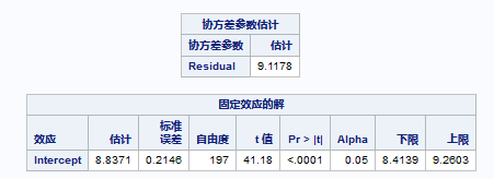
  • 零模型
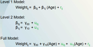
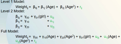
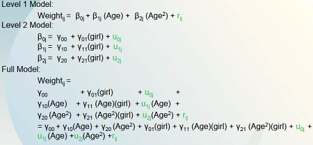
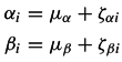
    • level1 model:Weight_ij=β_0j+r_ij
    • level2 model:β_0j=γ_0j+u_0j
    • full model:Weight_ij=γ_0j+u_0j+r_ij
 1
 2
 3
 4
 5
 6
 7
 8
 9
10
11
12
13
14
15
16
17
18
19
20
21
22
23
24
25
26
27
28
29
30
31
32
33
34
35
36
37
38
39
40
41
42
43
44
45
46
47
48
49
50
51
52
53
54
55
56
57
58
59
60
61
62

mixed weight || id:
est store model_0
esttab model_0,nogap

------------------------------------------------------------------------------
      weight |      Coef.   Std. Err.      z    P>|z|     [95% Conf. Interval]
-------------+----------------------------------------------------------------
       _cons |   8.837091   .2145919    41.18   0.000     8.416499    9.257683
------------------------------------------------------------------------------

------------------------------------------------------------------------------
  Random-effects Parameters  |   Estimate   Std. Err.     [95% Conf. Interval]
-----------------------------+------------------------------------------------
id: Identity                 |
                  var(_cons) |   4.11e-24   2.14e-23      1.53e-28    1.10e-19
-----------------------------+------------------------------------------------
               var(Residual) |   9.117835   .9163788      7.487599    11.10301
------------------------------------------------------------------------------
LR test vs. linear model: chibar2(01) = 2.3e-13       Prob >= chibar2 = 1.0000

estat icc

Intraclass correlation
------------------------------------------------------------------------------
                       Level |        ICC   Std. Err.     [95% Conf. Interval]
-----------------------------+------------------------------------------------
                          id |   4.50e-25          0      4.50e-25    4.50e-25
------------------------------------------------------------------------------

runmlwin weight cons, level2(id: cons) level1(newid: cons)

xtset id
xtreg weight,re mle

------------------------------------------------------------------------------
      weight |      Coef.   Std. Err.      z    P>|z|     [95% Conf. Interval]
-------------+----------------------------------------------------------------
       _cons |   8.837091   .2145884    41.18   0.000     8.416505    9.257676
-------------+----------------------------------------------------------------
    /sigma_u |          0   .3269978                             .           .
    /sigma_e |   3.019575   .1517333                      2.736359    3.332105
         rho |          0  (omitted)
------------------------------------------------------------------------------
LR test of sigma_u=0: chibar2(01) = 0.00               Prob >= chibar2 = 1.000


gllamm weight, i(id) 

------------------------------------------------------------------------------
      weight |      Coef.   Std. Err.      z    P>|z|     [95% Conf. Interval]
-------------+----------------------------------------------------------------
       _cons |   8.837091   .2145919    41.18   0.000     8.416499    9.257683
------------------------------------------------------------------------------
Variance at level 1
------------------------------------------------------------------------------
  9.1178355 (.91637695)
Variances and covariances of random effects
------------------------------------------------------------------------------
***level 2 (id)
    var(1): 9.541e-27 (6.388e-14)
------------------------------------------------------------------------------
  • SAS
1
2
3
4
5
6
7

proc mixed data=WORK.IMPORT method = ml;
      ID id;
      class id;
      model weight =  /solution CL;
      random intercept / sub=id;
run;

  • 线性增长曲线模型+随机截距模型
 1
 2
 3
 4
 5
 6
 7
 8
 9
10
11
12
13
14
15
16
17
18
19
20
21
22
23
24
25
26
27
28
29
30
31
32
33
34
35
36
37
38
39
40
41
42
43
44
45
46
47
48
49
50
51
52
53
54
55
56
57
58
59
60
61
62
63
64
65
66

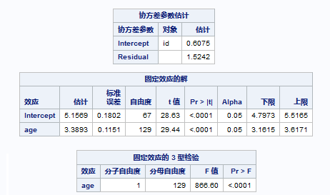
mixed weight age || id: , nolog
est store model_1
esttab model_1,nogap

------------------------------------------------------------------------------
      weight |      Coef.   Std. Err.      z    P>|z|     [95% Conf. Interval]
-------------+----------------------------------------------------------------
         age |   3.389281    .115129    29.44   0.000     3.163633     3.61493
       _cons |   5.156913    .180158    28.62   0.000      4.80381    5.510016
------------------------------------------------------------------------------

------------------------------------------------------------------------------
  Random-effects Parameters  |   Estimate   Std. Err.     [95% Conf. Interval]
-----------------------------+------------------------------------------------
id: Identity                 |
                  var(_cons) |   .6076662   .2040674      .3146395    1.173591
-----------------------------+------------------------------------------------
               var(Residual) |   1.524052   .1866496      1.198819    1.937518
------------------------------------------------------------------------------
LR test vs. linear model: chibar2(01) = 16.16         Prob >= chibar2 = 0.0000

xtreg weight age,re mle

------------------------------------------------------------------------------
      weight |      Coef.   Std. Err.      z    P>|z|     [95% Conf. Interval]
-------------+----------------------------------------------------------------
         age |   3.389281    .115221    29.42   0.000     3.163452     3.61511
       _cons |   5.156913   .1803058    28.60   0.000      4.80352    5.510306
-------------+----------------------------------------------------------------
    /sigma_u |   .7795294   .1308912                      .5609276    1.083324
    /sigma_e |   1.234525   .0755956                      1.094906    1.391947
         rho |   .2850594   .0795663                      .1521693     .456768
------------------------------------------------------------------------------
LR test of sigma_u=0: chibar2(01) = 16.16              Prob >= chibar2 = 0.000

gllamm weight age, i(id)

------------------------------------------------------------------------------
      weight |      Coef.   Std. Err.      z    P>|z|     [95% Conf. Interval]
-------------+----------------------------------------------------------------
         age |    3.38937   .1152127    29.42   0.000     3.163557    3.615183
       _cons |   5.155346   .1803718    28.58   0.000     4.801824    5.508868
------------------------------------------------------------------------------
Variance at level 1
------------------------------------------------------------------------------
  1.5238042 (.18694777)
Variances and covariances of random effects
------------------------------------------------------------------------------
***level 2 (id)
    var(1): .60524948 (.20137659)
------------------------------------------------------------------------------

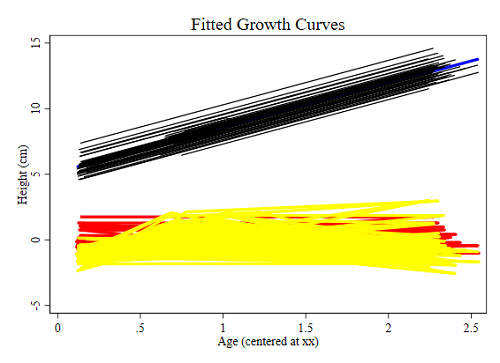
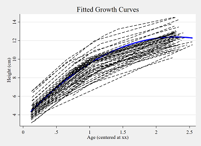
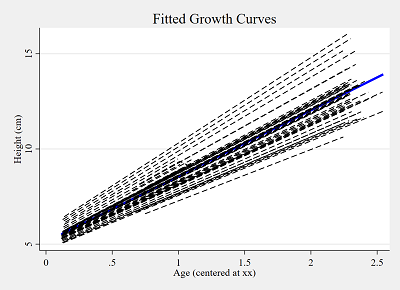
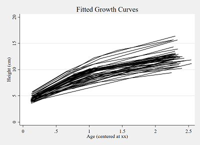
mixed weight age || id: , nolog
predict fv0, fitted
predict u0, reffects
predict resid, residual
sort id age
local model _b[_cons] + _b[age]*x
twoway (function y = `model',range(0.1149 2.5462) lw(thick) color(blue)) ///
       (line weight age,connect(ascending) lw(thick) color(green)) ///
       (line fv0 age,connect(ascending) color(black)) ///
       (line u0 age, lw(thick) color(red)) ///
       (line resid age, lw(thick) color(yellow)), ///
       xt(Age (centered at xx)) yt(Height (cm)) ///
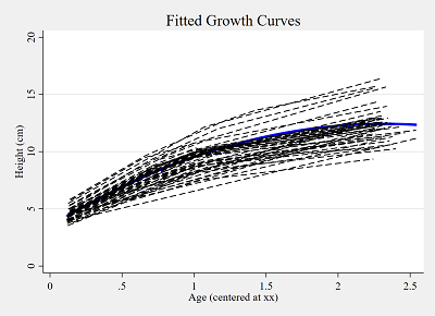
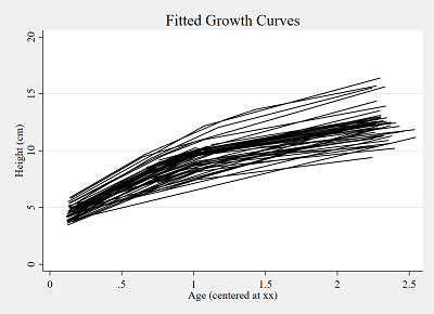
       legend(off) title(Fitted Growth Curves)
1
2
3
4
5
6

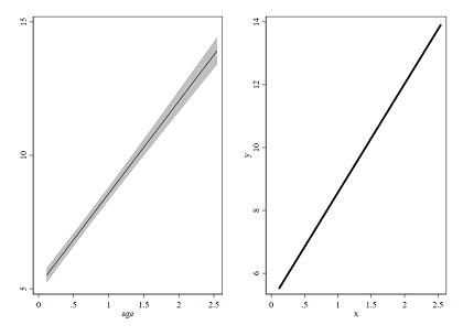
mixed weight age || id: , nolog
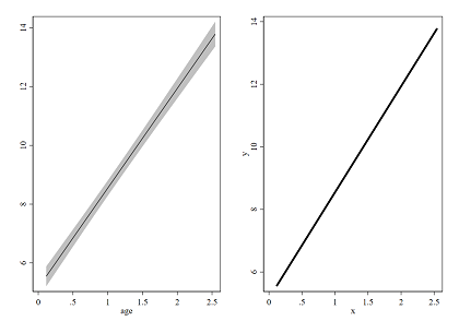
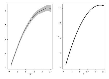
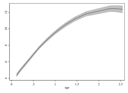
mcp2 age,ci name(age_mcp)
local model _b[_cons] + _b[age]*x
twoway (function y = `model',range(0.1149 2.5462) lw(thick) color(black)), name(age_function)
graph combine age_mcp age_function,row(1)

1
2
3
4
5
6
7
8
9

mixed weight c.age##c.age || id: , nolog
predict fv, fitted
sort id age
local model _b[_cons] + _b[age]*x + _b[c.age#c.age]*x^2
twoway (function y = `model',range(0.1149 2.5462) lw(thick) color(blue)) ///
       (line fv age,connect(ascending) color(black)), ///
       xt(Age (centered at xx)) yt(Height (cm)) ///
       legend(off) title(Fitted Growth Curves)
1
2
3
4
5
6

qui mixed weight c.age##c.age || id: , nolog
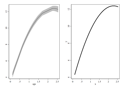
mcp2 age,ci name(age_mcp2)
local model _b[_cons] + _b[age]*x + _b[c.age#c.age]*x^2
twoway (function y = `model',range(0.1149 2.5462) lw(thick) color(black)),name(age_function2)
graph combine age_mcp2 age_function2,row(1)

  • SAS
1
2
3
4
5
6
7

proc mixed data=WORK.IMPORT method = ml;
      ID id;
      class id;
      model weight = age  /solution CL;
      random intercept / sub=id;
run;

  • 线性增长曲线模型+随机截距和随机斜率
 1
 2
 3
 4
 5
 6
 7
 8
 9
10
11
12
13
14
15
16
17
18
19
20
21
22
23
24
25
26
27
28
29
30
31
32

mixed weight age || id: age,  covariance(unstructured) nolog
est store model_2
esttab model_2,nogap

------------------------------------------------------------------------------
      weight |      Coef.   Std. Err.      z    P>|z|     [95% Conf. Interval]
-------------+----------------------------------------------------------------
         age |   3.459671   .1258877    27.48   0.000     3.212936    3.706406
       _cons |   5.110496   .1494781    34.19   0.000     4.817524    5.403468
------------------------------------------------------------------------------

------------------------------------------------------------------------------
  Random-effects Parameters  |   Estimate   Std. Err.     [95% Conf. Interval]
-----------------------------+------------------------------------------------
id: Unstructured             |
                    var(age) |   .2023919    .124311      .0607264     .674542
                  var(_cons) |   .0970272    .110823      .0103434    .9101719
              cov(age,_cons) |    .140134   .0566958      .0290123    .2512556
-----------------------------+------------------------------------------------
               var(Residual) |   1.357922   .1650528      1.070072    1.723204
------------------------------------------------------------------------------
LR test vs. linear model: chi2(3) = 27.38                 Prob > chi2 = 0.0000

mixed weight age || id: age,  covariance(unstructured) nolog
predict fv2, fitted
sort id age
local model2 _b[_cons] + _b[age]*x
twoway (function y = `model2',range(0.1149 2.5462) lw(thick) color(blue)) ///
       (line fv2 age,connect(ascending) color(black)), ///
       xt(Age (centered at xx)) yt(Height (cm)) ///
       legend(off) title(Fitted Growth Curves)

1
2
3
4
5
6

mixed weight age || id: age,  covariance(unstructured) nolog
mcp2 age,ci name(age_mcp3)
local model2 _b[_cons] + _b[age]*x
twoway (function y = `model2',range(0.1149 2.5462) lw(thick) color(black)) ,name(age_function3)
graph combine age_mcp3 age_function3,row(1)


  • SAS
1
2


  • 曲线增长模型+随机截距
 1
 2
 3
 4
 5
 6
 7
 8
 9
10
11
12
13
14
15
16
17
18
19
20
21
22
23
24
25
26
27
28
29
30
31
32
33
34
35
36
37
38
39
40
41
42
43
44
45
46
47
48
49
50
51
52
53
54
55
56
57
58
59
60
61
62
63
64
65
66
67
68
69
70
71
72
73
74
75
76
77
78
79
80
81
82
83
84
85
86
87
88

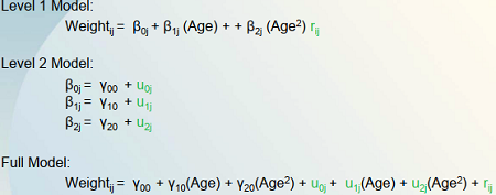
mixed weight age c.age#c.age || id: age, covariance(unstructured) nolog
est store model_3
esttab model_3,nogap

------------------------------------------------------------------------------
      weight |      Coef.   Std. Err.      z    P>|z|     [95% Conf. Interval]
-------------+----------------------------------------------------------------
         age |   7.703998   .2394082    32.18   0.000     7.234767    8.173229
 c.age#c.age |  -1.660465   .0885229   -18.76   0.000    -1.833967   -1.486963
       _cons |   3.494512   .1372636    25.46   0.000      3.22548    3.763544
------------------------------------------------------------------------------

------------------------------------------------------------------------------
  Random-effects Parameters  |   Estimate   Std. Err.     [95% Conf. Interval]
-----------------------------+------------------------------------------------
id: Unstructured             |
                    var(age) |    .254097   .0886513      .1282407    .5034696
                  var(_cons) |     .40444   .1645248      .1822168    .8976766
              cov(age,_cons) |   .0880873   .0880255     -.0844394    .2606141
-----------------------------+------------------------------------------------
               var(Residual) |   .3315169   .0582667      .2349093    .4678548
------------------------------------------------------------------------------
LR test vs. linear model: chi2(3) = 115.58                Prob > chi2 = 0.0000

Note: LR test is conservative and provided only for reference.


*比较三个模型
esttab model_1 model_2 model_3,nogap

------------------------------------------------------------
                      (1)             (2)             (3)   
                   weight          weight          weight   
------------------------------------------------------------
weight                                                      
age                 3.389***        3.460***        7.704***
                  (29.44)         (27.48)         (32.18)   
c.age#c.age                                        -1.660***
                                                 (-18.76)   
_cons               5.157***        5.110***        3.495***
                  (28.62)         (34.19)         (25.46)   
------------------------------------------------------------
lns1_1_1                                                    
_cons              -0.249          -0.799**        -0.685***
                  (-1.48)         (-2.60)         (-3.93)   
------------------------------------------------------------
lnsig_e                                                     
_cons               0.211***        0.153*         -0.552***
                   (3.44)          (2.52)         (-6.28)   
------------------------------------------------------------
lns1_1_2                                                    
_cons                              -1.166*         -0.453*  
                                  (-2.04)         (-2.23)   
------------------------------------------------------------
atr1_1_1_2                                                  
_cons                               9.593           0.282   
                                   (0.00)          (0.79)   
------------------------------------------------------------
N                     198             198             198   
------------------------------------------------------------
t statistics in parentheses
* p<0.05, ** p<0.01, *** p<0.001


lrtest model_0 model_1

Likelihood-ratio test                                 LR chi2(1)  =     16.16
(Assumption: model_0 nested in model_1)               Prob > chi2 =    0.0001

lrtest model_1 model_2

Likelihood-ratio test                                 LR chi2(2)  =     11.21
(Assumption: model_1 nested in model_2)               Prob > chi2 =    0.0037

lrtest model_2 model_3

Likelihood-ratio test                                 LR chi2(1)  =    169.28
(Assumption: model_2 nested in model_3)               Prob > chi2 =    0.0000

mixed weight age c.age#c.age || id: age, covariance(unstructured) nolog
predict fv3, fitted
sort id age
local model _b[_cons] + _b[age]*x + _b[c.age#c.age]*x^2
twoway (function y = `model',range(0.1149 2.5462) lw(thick) color(blue)) ///
       (line fv3 age,connect(ascending) color(black)), ///
       xt(Age (centered at xx)) yt(Height (cm)) ///
       legend(off) title(Fitted Growth Curves)

1
2
3
4
5
6

mixed weight age c.age#c.age || id: age, covariance(unstructured) nolog
mcp2 age,ci name(age_mcp4)
local model _b[_cons] + _b[age]*x + _b[c.age#c.age]*x^2
twoway (function y = `model',range(0.1149 2.5462) lw(thick) color(black)),name(age_function4)
graph combine age_mcp4 age_function4,row(1)

  • 男性与女性相同线性与曲线时间效应
 1
 2
 3
 4
 5
 6
 7
 8
 9
10
11
12
13
14
15
16
17
18
19
20
21
22
23
24
25
26
27
28
29
30
31
32
33
34
35
36
37
38
39
40
41
42
43
44

mixed weight age c.age#c.age i.girl || id: age, covariance(unstructured) nolog
est store model_4
esttab model_4,nogap

----------------------------
                      (1)   
                   weight   
----------------------------
weight                      
age                 7.698***
                  (32.32)   
c.age#c.age        -1.658***
                 (-18.83)   
0.girl                  0   
                      (.)   
1.girl             -0.596**
                  (-3.04)   
_cons               3.795***
                  (22.93)   
----------------------------
lns1_1_1                    
_cons              -0.674***
                  (-3.94)   
----------------------------
lns1_1_2                    
_cons              -0.520*  
                  (-2.40)   
----------------------------
atr1_1_1_2                  
_cons               0.158   
                   (0.48)   
----------------------------
lnsig_e                     
_cons              -0.558***
                  (-6.44)   
----------------------------
N                     198   
----------------------------
t statistics in parentheses
* p<0.05, ** p<0.01, *** p<0.001

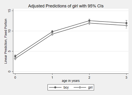
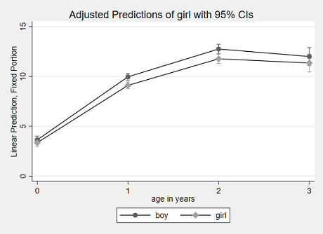
margins i.girl, at(age=(0(1)3)) vsquish
marginsplot, name(model_4, replace) x(age)
1
2
3
4
5
6
7

mixed weight age c.age#c.age i.girl || id: age, covariance(unstructured) nolog
predict fv4, fitted
sort id age
twoway (line fv4 age,connect(ascending) color(black)), ///
       xt(Age (centered at xx)) yt(Height (cm)) ///
       legend(off) title(Fitted Growth Curves)
1
2
3

mixed weight age c.age#c.age i.girl || id: age, covariance(unstructured) nolog
mcp2 age,ci name(age_mcp5)

  • 男性与女性不同线性与曲线时间效应
 1
 2
 3
 4
 5
 6
 7
 8
 9
10
11
12
13
14
15
16
17
18
19
20
21
22
23
24
25
26
27
28
29
30
31
32
33
34
35
36
37
38
39
40
41
42
43
44
45
46
47

mixed weight i.girl##c.age##c.age|| id: age, covariance(unstructured) nolog
est store model_5
esttab model_5,nogap

----------------------------
                      (1)   
                   weight   
----------------------------
weight                      
1.girl             -0.288   
                  (-1.08)   
age                 8.089***
                  (24.65)   
1.girl#c.age       -0.798   
                  (-1.69)   
c.age#c.age        -1.767***
                 (-14.58)   
1.girl#c.a~e        0.225   
                   (1.29)   
_cons               3.645***
                  (19.56)   
----------------------------
lns1_1_1                    
_cons              -0.709***
                  (-4.03)   
----------------------------
lns1_1_2                    
_cons              -0.517*  
                  (-2.42)   
----------------------------
atr1_1_1_2                  
_cons               0.186   
                   (0.55)   
----------------------------
lnsig_e                     
_cons              -0.564***
                  (-6.51)   
----------------------------
N                     198   
----------------------------
t statistics in parentheses
* p<0.05, ** p<0.01, *** p<0.001


margins i.girl, at(age=(0(1)3)) vsquish
marginsplot, name(model_5, replace) x(age)
1
2
3
4
5
6
7

mixed weight i.girl##c.age##c.age|| id: age, covariance(unstructured) nolog
predict fv5, fitted
sort id age
twoway (line fv5 age,connect(ascending) color(black)), ///
       xt(Age (centered at xx)) yt(Height (cm)) ///
       legend(off) title(Fitted Growth Curves)

1
2
3
4
5
6

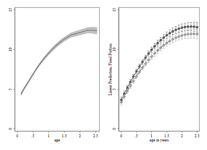
mixed weight i.girl##c.age##c.age|| id: age, covariance(unstructured) nolog
mcp2 age,ci name(age_mcp6) areaopts(ylabel(0(5)15))
margins girl, at(age=(0(0.1)2.5))
marginsplot,name(age_mcp7) legend(off) title("")
graph combine age_mcp6 age_mcp7,col(2)


  • 增长曲线模型总结
    • 增长曲线模型对个体随时间变化进行描述和解释的技术
    • 增长曲线模型需要至少三期面板数据
    • 如果结果变量是非连续型变量,则需要更加复杂的增长曲线模型
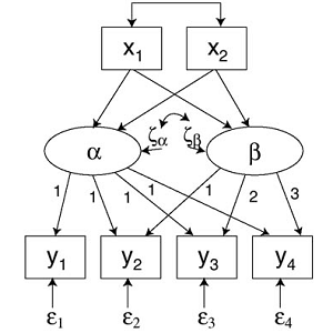
    • 增长曲线模型可以通过结构方程模型的方式来估计。如果想要包含测量模型或中介效应,结构方程模型估计更好!

  • 无条件增长曲线模型与条件增长曲线模型
    • 增长曲线模型既可以视为多层次(层级)模型的特例,也可以视为结构方程模型的特例
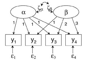
    • 无条件模型(unconditional model)
      • 无条件增长曲线模型:对单一结果的重复测量,并对该变量的轨迹建模
      • 无条件模型的SEM
    • 条件模型(conditional model)
      • 条件增长曲线模型:层一方程与无条件模型一样,层二方程加入影响截距和斜率的变量,两者影响了随时间变化的轨迹(over-time trajectories)
      • 条件模型的SEM

 1
 2
 3
 4
 5
 6
 7
 8
 9
10
11
12
13
14
15
16
17
18
19
20
21
22
23
24
25
26
27
28
29
30
31
32
33
34
35
36
37

use "D:\Data Storages\Dataset for Learning\depression_clean.dta",clear
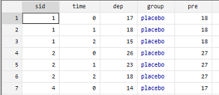
reshape long dep, i(sid) j(time)
mixed dep time || sid:time, cov(unstr)
est store mix1
esttab mix1,nogap

----------------------------
                      (1)   
                      dep   
----------------------------
dep                         
time               -1.602***
                  (-3.76)   
_cons               14.19***
                  (17.42)   
----------------------------
lns1_1_1                    
_cons               0.582   
                   (1.82)   
----------------------------
lns1_1_2                    
_cons               1.544***
                  (10.24)   
----------------------------
atr1_1_1_2                  
_cons              -0.139   
                  (-0.47)   
----------------------------
lnsig_e                     
_cons               1.167***
                  (11.19)   
----------------------------
N                     138   
----------------------------
t statistics in parentheses
* p<0.05, ** p<0.01, *** p<0.001
    • 用SEM模式来估计
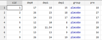
    • 转为宽格式
 1
 2
 3
 4
 5
 6
 7
 8
 9
10
11
12
13
14
15
16
17
18
19
20
21
22
23
24
25
26
27
28
29
30
31
32
33
34

reshape wide
sem (dep0 <- I@1 S@0 _cons@0) ///
    (dep1 <- I@1 S@1 _cons@0) ///
    (dep2 <- I@1 S@2 _cons@0), /// 
    var(e.dep0@var e.dep1@var e.dep2@var) means(I S)
est store sem1
esttab sem1,nogap

----------------------------
                      (1)   
----------------------------
/                           
mean(I)             14.19***
                  (17.42)   
mean(S)            -1.602***
                  (-3.76)   
var(e.dep0)         10.31***
                   (4.80)   
var(e.dep1)         10.31***
                   (4.80)   
var(e.dep2)         10.31***
                   (4.80)   
var(I)              21.94***
                   (3.32)   
var(S)              3.201   
                   (1.56)   
cov(I,S)           -1.154   
                  (-0.42)   
----------------------------
N                      46   
----------------------------
t statistics in parentheses
* p<0.05, ** p<0.01, *** p<0.001
    • 增加非时变变量
    • 用混合模型来估计
 1
 2
 3
 4
 5
 6
 7
 8
 9
10
11
12
13
14
15
16
17
18
19
20
21
22
23
24
25
26
27
28
29
30
31
32
33
34
35
36
37
38

reshape long dep, i(sid) j(time)
mixed dep time pre || sid:time, var cov(unstr)
est store mix2
esttab mix2,nogap

----------------------------
                      (1)   
                      dep   
----------------------------
dep                         
time               -1.602***
                  (-3.76)   
pre                 0.505**
                   (2.66)   
_cons               3.565   
                   (0.88)   
----------------------------
lns1_1_1                    
_cons               0.582   
                   (1.82)   
----------------------------
lns1_1_2                    
_cons               1.510***
                   (9.72)   
----------------------------
atr1_1_1_2                  
_cons              -0.290   
                  (-1.01)   
----------------------------
lnsig_e                     
_cons               1.167***
                  (11.19)   
----------------------------
N                     138   
----------------------------
t statistics in parentheses
* p<0.05, ** p<0.01, *** p<0.001
    • 用SEM来估计
 1
 2
 3
 4
 5
 6
 7
 8
 9
10
11
12
13
14
15
16
17
18
19
20
21
22
23
24
25
26
27
28
29
30
31
32
33
34
35
36
37
38
39
40
41
42
43
44
45
46
47

reshape wide
sem (dep0 <- I@1 S@0 pre@p1 _cons@0)  ///
    (dep1 <- I@1 S@1 pre@p1 _cons@0)  ///
    (dep2 <- I@1 S@2 pre@p1 _cons@0), ///
    var(e.dep0@var e.dep1@var e.dep2@var)  ///
    means(I S) covar(pre*I@0 pre*S@0)
est store sem2
esttab sem2,nogap

----------------------------
                      (1)   
----------------------------
dep0                        
pre                 0.505**
                   (2.60)   
----------------------------
dep1                        
pre                 0.505**
                   (2.60)   
----------------------------
dep2                        
pre                 0.505**
                   (2.60)   
----------------------------
/                           
mean(I)             3.565   
                   (0.86)   
mean(S)            -1.602***
                  (-3.76)   
var(e.dep0)         10.31***
                   (4.80)   
var(e.dep1)         10.31***
                   (4.80)   
var(e.dep2)         10.31***
                   (4.80)   
var(I)              20.51**
                   (3.22)   
var(S)              3.201   
                   (1.56)   
cov(I,S)           -2.289   
                  (-0.82)   
----------------------------
N                      46   
----------------------------
t statistics in parentheses
* p<0.05, ** p<0.01, *** p<0.001
    • 非时变变量与时间的交互项
    • 用混合模型估计
 1
 2
 3
 4
 5
 6
 7
 8
 9
10
11
12
13
14
15
16
17
18
19
20
21
22
23
24
25
26
27
28
29
30
31
32
33
34
35
36
37
38
39
40

reshape long
mixed dep c.time##c.pre || sid:time, var cov(unstr)
est store mix3
esttab mix3,nogap

----------------------------
                      (1)   
                      dep   
----------------------------
dep                         
time               -5.095*  
                  (-2.11)   
pre                 0.357   
                   (1.66)   
c.time#c.pre        0.166   
                   (1.47)   
_cons               6.676   
                   (1.45)   
----------------------------
lns1_1_1                    
_cons               0.520   
                   (1.48)   
----------------------------
lns1_1_2                    
_cons               1.503***
                   (9.69)   
----------------------------
atr1_1_1_2                  
_cons              -0.265   
                  (-0.89)   
----------------------------
lnsig_e                     
_cons               1.167***
                  (11.19)   
----------------------------
N                     138   
----------------------------
t statistics in parentheses
* p<0.05, ** p<0.01, *** p<0.001
    • 用SEM估计
 1
 2
 3
 4
 5
 6
 7
 8
 9
10
11
12
13
14
15
16
17
18
19
20
21
22
23
24
25
26
27
28
29
30
31
32
33
34
35
36
37
38
39
40
41
42
43

reshape wide
sem (dep0 <- I@1 S@0 _cons@0) ///
    (dep1 <- I@1 S@1 _cons@0) ///
    (dep2 <- I@1 S@2 _cons@0) ///
    (I <- pre _cons) (S <- pre _cons), ///
    var(e.dep0@var e.dep1@var e.dep2@var) covar(e.I*e.S)
est store sem3
esttab sem3,nogap

----------------------------
                      (1)   
----------------------------
I                           
pre                 0.357   
                   (1.66)   
_cons               6.676   
                   (1.45)   
----------------------------
S                           
pre                 0.166   
                   (1.47)   
_cons              -5.095*  
                  (-2.11)   
----------------------------
/                           
var(e.dep0)         10.31***
                   (4.80)   
var(e.dep1)         10.31***
                   (4.80)   
var(e.dep2)         10.31***
                   (4.80)   
var(e.I)            20.21**
                   (3.22)   
var(e.S)            2.828   
                   (1.43)   
cov(e.I,e.S)       -1.957   
                  (-0.73)   
----------------------------
N                      46   
----------------------------
t statistics in parentheses
* p<0.05, ** p<0.01, *** p<0.001
    • 增加时变变量
    • 用混合模型估计
 1
 2
 3
 4
 5
 6
 7
 8
 9
10
11
12
13
14
15
16
17
18
19
20
21
22
23
24
25
26
27
28
29
30
31
32
33
34
35
36
37
38

use "D:\Data Storages\Dataset for Learning\lsay_long_clean.dta",clear
mixed math c.yr c.att || id:yr, var cov(unstr)
est store mix4
esttab mix4,nogap

----------------------------
                      (1)   
                     math   
----------------------------
math                        
yr                  2.643***
                  (48.36)   
att                 0.170***
                   (6.72)   
_cons               54.68***
                 (164.16)   
----------------------------
lns1_1_1                    
_cons               0.604***
                  (13.36)   
----------------------------
lns1_1_2                    
_cons               2.353***
                 (178.61)   
----------------------------
atr1_1_1_2                  
_cons           -0.000560   
                  (-0.02)   
----------------------------
lnsig_e                     
_cons               1.337***
                 (113.17)   
----------------------------
N                   10785   
----------------------------
t statistics in parentheses
* p<0.05, ** p<0.01, *** p<0.001
    • 用SEM估计
 1
 2
 3
 4
 5
 6
 7
 8
 9
10
11
12
13
14
15
16
17
18
19
20
21
22
23
24
25
26
27
28
29
30
31
32
33
34
35
36
37
38
39
40
41
42
43
44
45
46
47
48
49
50
51
52
53
54
55
56
57
58

reshape wide math att, i(id) j(yr)
sem (math0 <- I@1 S@0  _cons@0) ///
    (math1 <- I@1 S@1  _cons@0) ///
    (math2 <- I@1 S@2  _cons@0), ///
    var(e.math0@var e.math1@var e.math2@var) ///
    means(I S)
    mat b = e(b)

sem (math0 <- I@1 S@0 att0@b1 _cons@0) ///
    (math1 <- I@1 S@1 att1@b1 _cons@0) ///
    (math2 <- I@1 S@2 att2@b1 _cons@0), ///
    var(e.math0@var e.math1@var e.math2@var) ///  
    means(I S) ///
    covar(att0*I@0 att1*I@0 att2*I@0) ///
    covar(att0*S@0 att1*S@0 att2*S@0) ///
    from(b)

est store sem4
esttab sem4,nogap

----------------------------
                      (1)   
----------------------------
math0                       
att0                0.170***
                   (6.68)   
----------------------------
math1                       
att1                0.170***
                   (6.68)   
----------------------------
math2                       
att2                0.170***
                   (6.68)   
----------------------------
/                           
mean(I)             54.68***
                 (163.55)   
mean(S)             2.643***
                  (48.36)   
var(e.math0)        14.50***
                  (42.32)   
var(e.math1)        14.50***
                  (42.32)   
var(e.math2)        14.50***
                  (42.32)   
var(I)              110.5***
                  (37.96)   
var(S)              3.349***
                  (11.05)   
cov(I,S)          -0.0108   
                  (-0.02)   
----------------------------
N                    3595   
----------------------------
t statistics in parentheses
* p<0.05, ** p<0.01, *** p<0.001

1
2
3
4
5
6
7

cd "D:\Data Storages\Dataset for Learning\mlmus3"
use asian.dta,clear
label def gender 1 "male" 2 "female"
label val gender gender
sort id age
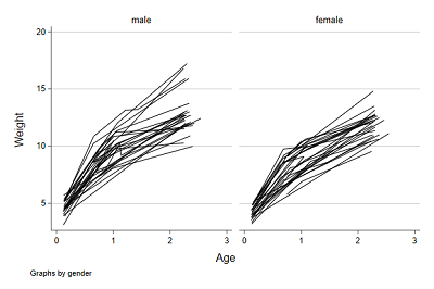
graph twoway (line weight age, connect(ascending)),by(gender) xtitle(Age) ytitle(Weight)

  • 可见体重增长并非是线性,早期是快速,后期放缓
  • 我们首先通过在模型中包括年龄的二次项来建模增长轨迹的非线性,并给出二阶多项式。
    • 并且在任何给定年龄,男孩和女孩的平均体重都会有所不同,而其初始体重和生长速度会有所不同。
    • 建立模型:
    • y是体重,w是性别,t是年龄, ζ1是随机截距, ζ2是随机系数
 1
 2
 3
 4
 5
 6
 7
 8
 9
10
11
12
13
14
15
16
17
18
19
20
21
22
23
24
25
26
27
28
29
30
31
32
33
34
35
36
37
38
39
40
41

recode gender (2=1 "female") (1=0 "male"), generate(sex)
gen age2 = age^2
xtmixed weight sex age age2 || id: age, covariance(unstructured) mle
est store m1
esttab m1,nogap se

----------------------------
                      (1)   
                   weight   
----------------------------
weight                      
sex                -0.596**
                  (0.196)   
age                 7.698***
                  (0.238)   
age2               -1.658***
                 (0.0881)   
_cons               3.795***
                  (0.166)   
----------------------------
lns1_1_1                    
_cons              -0.674***
                  (0.171)   
----------------------------
lns1_1_2                    
_cons              -0.520*  
                  (0.217)   
----------------------------
atr1_1_1_2                  
_cons               0.158   
                  (0.332)   
----------------------------
lnsig_e                     
_cons              -0.558***
                 (0.0867)   
----------------------------
N                     198   
----------------------------
Standard errors in parentheses
* p<0.05, ** p<0.01, *** p<0.001